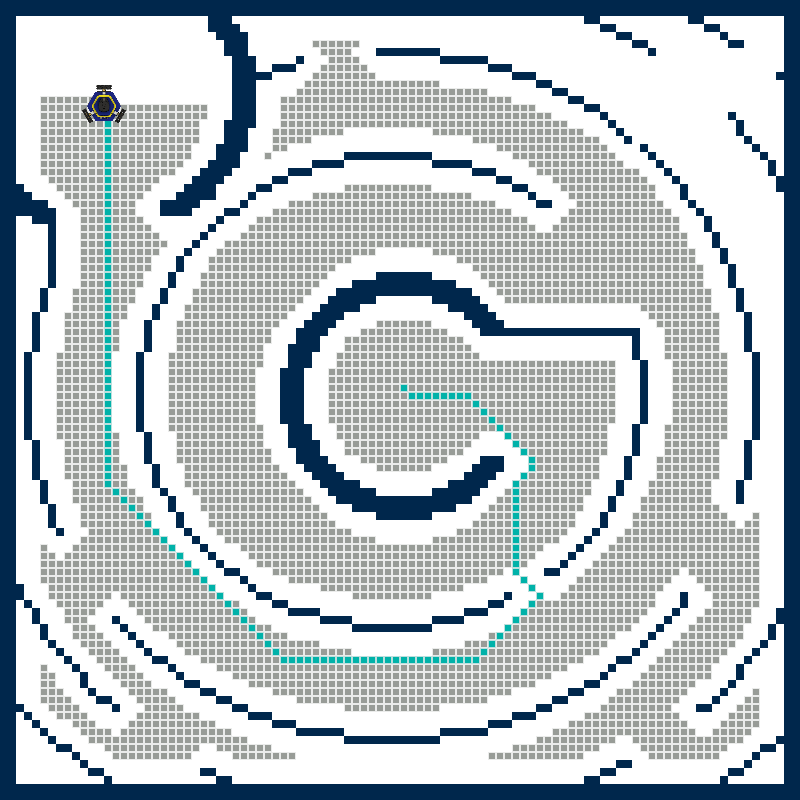
In this project, we will write a path planning algorithm, which will find a path to any goal in a map. When you've completed the project, you'll be able to find paths like this one:
- Getting the Code
- Project Description
- Advanced Extensions
- Code Overview
- Task Summary
- Advanced Extension: Distance Transform
Read these instructions for:
Getting the Code
To get the template code for this project, see your course page for the GitHub Classroom assignment link.
You should always sign the license for your code by editing the file LICENSE.txt. Replace <COPYRIGHT HOLDER> with the names of all teammates, separated by commas. Replace <YEAR> with the current year.
-
P3.0:
In the file
LICENSE.txt, replace<COPYRIGHT HOLDER>with the names of all teammates, separated by commas. Replace<YEAR>with the current year.
Editing the code on Replit
Much of the code for this project can be run without using the robot, using a webapp we have made for testing your code. When your code is working, you can then run it on the robot.
You can use Replit to run your code by connecting your code repository to a Repl. Instructions are available on the Replit website.
Warning: Make sure you are following your class regulations regarding public code if using Replit. Replit free accounts only allow public projects, which would make your project code accessible to anyone on the internet. Follow your instructor's guidance for running this code locally.
Project Description
We will implement Breadth First Search within robot maps. We also provide an advanced extension to implement the A-Star search algorithm, as discussed in lecture.
To help you develop your algorithm, we have created a webapp which you can use to test your algorithm. You can find a tutorial on how to use it here. The code can be run in Replit for testing purposes, using provided test maps, or maps that you have downloaded from the robot. It will output a file that you can use in the webapp to visualize your code. Once your planning algorithm is working, you can run it on your robot using a real robot map.
Grid Graph
Information about the map for a particular environment is stored in a provided structclass called GridGraph, described in the code overview. You can visualize the available maps using the webapp.
A number of helper functions are available for you to use. Review them in the code overview.
You will need to complete the function findNeighbors()graph.find_neighbors().
The neighbors of a cell are the adjacent cells in the graph.
This function will be necessary in order to complete your planning algorithm.
-
P3.1:
In the file
graph_utils.cpp, complete functionfindNeighbors(). It should accept the index of a node and return a vector of indices of neighboring nodes. You may use either 4-connected or 8-connected neighbors. In the filesrc/graph.py, complete functiongraph.find_neighbors(). It should accept the cell coordinates of a node and return a list of neighboring cells. You may use either 4-connected or 8-connected neighbors.
-
Hint:
You might find the functions
idxToCell()andcellToIdx()helpful.
Storing Node Data
In order to perform graph search, we need to keep track of a few things for each cell:
- The cell's parent along the current path,
- The distance from the start node to the cell along the current path,
- Whether the cell has been visited.
Using the concepts we have learned so far, design code to store this data. Then, modify GridGraph to store the node information. You may extend your implementation to store any additional information you need.
Note: The nodes should be indexed the same way as the cells, as a single vector. You can use the cellToIdx() and idxToCell() functions to access node data for a specific cell.
-
P3.2:
In the
graph_utils.hsrc/graph.pyfile, design a data structure to store the cell information and modifyGridGraphto add any new member variables accordingly. -
P3.3:
In the
graph_utils.cppfile, complete functioninitGraph()to initialize the cell data. You can assume the graph will be loaded when the function is called. In thesrc/graph.pyfile, complete functiongraph.init_graph()to initialize the cell data. You can assume the graph will be loaded when the function is called. -
P3.4:
In the
graph_utils.cppfile, complete functiongetParent()so it returns the index of the parent of the given cell. If a cell does not have a parent, it should return -1. In thesrc/graph.pyfile, complete functiongraph.get_parent()so it returns a cell corresponding to the parent of the given cell. If a cell does not have a parent, it should return None.
-
Hint:
You might consider implementing a struct to represent your cell node and store a vector of cell node structs in
GridGraph. Alternatively, you might consider adding a few vectors to theGridGraphstruct to store the relevant information. You might consider implementing a class to represent your cell node and store a list of cell node objects inGridGraph. Alternatively, you might consider adding a few NumPy matrices to theGridGraphclass to store the relevant information. - Hint: The start node and unexplored nodes should not have parents.
Breadth First Search
In this section, you will write code to implement a Breadth First Search (BFS) over a graph, given a start and goal cell. You will write your code in the file src/graph_search/graph_search.cpp
src/graph_search.py. Your code should go in the function breadthFirstSearch()
breadth_first_search(), which looks like this:
std::vector breadthFirstSearch(GridGraph& graph, const Cell& start, const Cell& goal)
{
std::vector| path; // The final path should be placed here.
initGraph(graph); // Make sure all the node values are reset.
int start_idx = cellToIdx(start.i, start.j, graph);
/**
* TODO (P3): Implement BFS.
*/
return path;
} | | def breadth_first_search(graph, start, goal):
"""Breadth First Search (BFS) algorithm.
Args:
graph: The graph class.
start: Start cell as a Cell object.
goal: Goal cell as a Cell object.
"""
graph.init_graph() # Make sure all the node values are reset.
"""TODO (P3): Implement BFS."""
# If no path was found, return an empty list.
return []
Assume the graph is loaded with the corresponding map data. The function first calls initGraph()graph.init_graph() to make sure that all the nodes are initialized. The start and goal position are passed in as Cell types.Cell has two integer member variables: i and j, corresponding to the x-axis (column) and y-axis (row) coordinates of the cell. When the path is found, your code should store the path in the provided vector, path. You can use the provided function tracePath()trace_path(), as follows:
path = tracePath(goal_idx, graph);where goal_idx is an integer value which stores the index of the goal. If you have correctly maintained the parent structure of the cells and the idxToCell() and getParent() functions are implemented, this will return the path to the start node. The start node should not have a parent. If no path was found, your code should return an empty vector. Use checkCollision() to check whether a cell is in collision.
trace_path(goal_cell, graph)where goal_cell is a Cell corresponding to the goal. If you have correctly maintained the parent structure of the cells and graph.get_parent() function is implemented, this will return the path to the start node. The start node should not have a parent. If no path was found, your code should return an empty list. Use check_collision() to check whether a cell is in collision.
The webapp allows you to play back which cells are visited in your algorithm. It will show visited cells in grey so you can visualize the order that the cells are explored. To visualize the visited cells, you should add the cell to
the vector graph.visited_cells, as follows (given that the current cell is stored in Cell struct c)the list graph.visited_cells, as follows (given that the current cell is stored in Cell object c):
graph.visited_cells.push_back(c);graph.visited_cells.append(Cell(c.i, c.j))-
P3.5:
In the
graph_search.cppfile, implement Breadth First Search in functionbreadthFirstSearch(). In thegraph_search.pyfile, implement Breadth First Search in functionbreadth_first_search().
- Hint: BFS maintains a list of nodes to visit using a First-In-First-Out data structure (or a queue). C++ has a queue implementation called
std::queue. Assuming you have a queueq,q.push(my_node_idx)will push a value onto the back of the queue,q.front()will return the value at the front of the queue, andq.pop()will remove the first element of the queue. - Hint: Your visit list should store integers corresponding to the indices of the nodes of interest. You can use these indices to retrieve and modify cell data directly in the graph. Do not push any structs your graph stores onto the visit list! This makes a
copy of the data, so any changes you make would not be reflected in the graph. - Hint: You should not add any cells which are in collision to your visit list.
- Hint:If you complete the Distance Transform advanced extension, you can use
checkCollisionFast()to check collisions. This requires that you call your distance transform function first. The results will be slightly different thancheckCollision()if you use the Manhattan distance transform, but both are valid.
- Hint: BFS maintains a list of nodes to visit using a First-In-First-Out data structure (or a queue). In Python, you can use a regular list as a queue. Assuming you have a list
q,q.pop(0)will remove the value at the front of the queue and return it. - Hint: Your visit list can store node objects directly. Modifying them will modify the values everywhere in the graph, since Python objects are handled as references.
- Hint: You should not add any cells which are in collision to your visit list.
Path Planning on the Robot
You will write code to search for and drive along a path on the robot in the file src/robot_plan_path.cpprobot_plan_path.py. We use the MBot API to send the robot a path to follow. Modify the provided code template to call your path planning algorithm and then send the path to the robot. It will look something like this:
Note: The utility function loadFromFile() initializes the radius for collision checking to the robot radius, stored in variable ROBOT_RADIUS, plus the width of one cell. You might want to make the collision radius larger on the robot, so that your planner is more conservative on the robot.
To do this modify the value of graph.collision_radius after the map is loaded.
To do this, use the -r argument on the command line or change the default collision radius in the code.
-
P3.6:
In the
robot_plan_path.cppfile, call your path planning function and use theMBot::drivePath()function in the API to send the path to the robot. In therobot_plan_path.pyfile, call your path planning function and use theMBot.drive_path()function in the API to send the path to the robot.
- Hint: If you are using the
checkCollisionFast()function in your graph search, do not forget to call your distance transform function after the map is loaded. - Hint: The provided function
drivePath()returns immediately after sending the path command to motion controller. That means your program will quit before the robot has reached the goal. If you wish to send another path to the robot or perform some processing when the robot has reached the goal, you can write code to wait until the robot has reached the goal before finishing.
- Hint: The
MBot.drive_path()function returns immediately after sending the path command to motion controller. That means your program will quit before the robot has reached the goal. If you wish to send another path to the robot or perform some processing when the robot has reached the goal, you can write code to wait until the robot has reached the goal before finishing.
Before you run the code, you should make a map of the environment you want to run in (see the mapping tutorial). Once you have made a map, switch the robot into localization only mode.
To compile and run path planning on the robot, connect to the robot using VSCode. Then, from inside the repository you cloned onto the robot, compile as follows:
cd build
cmake -DMBOT=On ..
make
Do not forget the argument -DMBOT=On when running CMake. This is how the compiler knows whether to compile the robot code (which is not compiled by default for testing in Replit). To run the planning algorithm, in the build folder where you compiled, do:
./robot_plan_path [PATH/TO/MAP] [goal_x] [goal_y]The map is stored in ~/current.map. Use that path if you did not move the map since creating it. You can also pass in goal_x and goal_y, the global position of the goal, relative to the starting position of your map, in meters. If you do not pass these in, they will default to zero.
When you pass in arguments to the code, do not include the square brackets.
To run your code on the robot, do:
python robot_plan_path.py --goal [GOAL_x GOAL_y]The goal is an x and y position in meters. Use the robot's web app to pick a good goal by clicking the cell you want to navigate to and noting its coordinates.
Advanced Extensions
A-Star Search
As an advanced extension, you may write code to implement A-Star Search over a graph, given a start and goal cell. You will write your code in the file src/graph_search/graph_search.cppsrc/graph_search.py. Your code should go in the function aStarSearch()a_star_search(). This function looks a lot like the one for BFS. However, you will need to maintain the f-score of the nodes you explore. Modify your cell node data to include the f-score of the node.
In the graph_utils.cpp file, implement the function getScore() to return a double corresponding to the f-score of the given cell index.
In A-Star, the next node to explore is the one with the findLowestScore() takes a std::vector of integers as an argument, along with the graph, and returns the index of the lowest score node
int min_score_idx = findLowestScore(visit_list, graph);
int current = visit_list[min_score_idx];
visit_list.erase(visit_list.begin() + min_score_idx);-
Advanced Extension P3.i (1 extension point):
In the
graph_search.cppfile, implement A-Star Search in functionaStarSearch(). In thegraph_search.pyfile, implement A-Star Search in functiona_star_search().
Code Overview
See the documentation in the template code.
The following structs are provided:
-
Cell: For representing a cell in the graph.
wherestruct Cell { float i, j; };iis the row of the cell, andjis the column of the cell. -
GridGraph: For storing map data.
The member variablesstruct GridGraph { int width, height; // Width and height of the map in cells. float origin_x, origin_y; // The (x, y) coordinate corresponding to cell (0, 0) in meters. float meters_per_cell; // Width of a cell in meters. float collision_radius; // The radius to use to check collisions. int8_t threshold; // Threshold to check if a cell is occupied or not. std::vector<int8_t> cell_odds; // The odds that a cell is occupied. std::vector<float> obstacle_distances; // The distance from each cell to the nearest obstacle. };widthandheightstore the graph width and height, in cells. The variablesorigin_xandorigin_ycorrespond to the global position in meters of the cell(0, 0). This allows us to determine where the origin of the map is. The variablemeters_per_cellcontains the size of each cell, in meters. Finally, thecell_oddsvariable is a vector containing the odds value of each cell. The odds value and organization of the graph was covered in Lab 4.
Provided Utility Functions
This section describes functions which are useful for interacting with the graph, from the header include/autonomous_navigation/utils/graph_utils.h (implemented in src/utils/graph_utils.cpp). Other than those marked, these are implemented for you.
-
int cellToIdx(int i, int j, const GridGraph& graph): Given a cell rowiand columnjin the graph, calculates the index where the data for the cell is stored. -
Cell idxToCell(int idx, const GridGraph& graph): Given an index, calculates the corresponding cell rowiand columnjin the graph. -
Cell posToCell(float x, float y, const GridGraph& graph): Given a global positionxandy, in meters, calculates the corresponding cell in the graph. -
std::vector: Given a cell in the graph, calculates the corresponding global position in meters.cellToPos(int i, int j, const GridGraph& graph) -
bool loadFromFile(const std::string& file_path, GridGraph& graph): Loads graph data from a file. Also initializes the distance transform values to all zeros and calls theinitGraph()function. -
void initGraph(GridGraph& graph): (TODO, see Part 1) Initializes the graph data.
Note: This function should not modifygraph.obstacle_distances. -
std::vector: (TODO) Returns a list of the indices of the neighbors of the cell at a given index in the graph.findNeighbors(int idx, const GridGraph& graph)
-
bool checkCollisionFast(int idx, const GridGraph& graph): Uses the distance transform values to check whether visiting the cell atidxwould result in a collision.
Warning: This only works if the distance transform values are stored ingraph.obstacle_distances. When using the web app, the functiondistanceTransform()will be called when the map is loaded. -
bool checkCollision(int idx, const GridGraph& graph): Manually checks in a radius around the given cell for collisions.
Warning: This version does not require the distance transform but will be slower than the above version. -
int getParent(int idx, const GridGraph& graph): (TODO, see Part 1) Returns the index of the parent of the node atidx. -
float getScore(int idx, const GridGraph& graph): (TODO, A-Star only, see Advanced Extension: A-Star) Returns the f-score of the node atidx. -
std::vector<Cell> tracePath(int goal, const GridGraph& graph): Returns the path from the start cell to the given goal cell.
Warning: This only works ifgetParent()is implemented. -
int findLowestScore(const std::vector<int>& node_list, const GridGraph& graph): Returns the index of the node with the lowest f-score.
Warning: This only works ifgetScore()is implemented (A-Star only).
Task Summary
-
P3.1:
In the file
graph_utils.cpp, complete functionfindNeighbors(). It should accept the index of a node and return a vector of indices of neighboring nodes. You may use either 4-connected or 8-connected neighbors. In the filesrc/graph.py, complete functiongraph.find_neighbors(). It should accept the cell coordinates of a node and return a list of neighboring cells. You may use either 4-connected or 8-connected neighbors. -
P3.2:
In the
graph_utils.hsrc/graph.pyfile, design a data structure to store the cell information and modifyGridGraphto add any new member variables accordingly. -
P3.3:
In the
graph_utils.cppfile, complete functioninitGraph()to initialize the cell data. You can assume the graph will be loaded when the function is called. In thesrc/graph.pyfile, complete functiongraph.init_graph()to initialize the cell data. You can assume the graph will be loaded when the function is called. -
P3.4:
In the
graph_utils.cppfile, complete functiongetParent()so it returns the index of the parent of the given cell. If a cell does not have a parent, it should return -1. In thesrc/graph.pyfile, complete functiongraph.get_parent()so it returns a cell corresponding to the parent of the given cell. If a cell does not have a parent, it should return None. -
P3.5:
In the
graph_search.cppfile, implement Breadth First Search in functionbreadthFirstSearch(). In thegraph_search.pyfile, implement Breadth First Search in functionbreadth_first_search(). -
P3.6:
In the
robot_plan_path.cppfile, call your path planning function and use theMBot::drivePath()function in the API to send the path to the robot. In therobot_plan_path.pyfile, call your path planning function and use theMBot.drive_path()function in the API to send the path to the robot.
Advanced Extensions
If you want to go even further, you can implement the distance transform for faster collision checking. Template code for this extension is only available in C++, but you can implement it yourself in Python.
Distance Transform (Manhattan)
A binary distance transform calculates the distance from each cell to the nearest occupied cell in a map. We can use this to check whether a cell is in collision quickly. The distance transform values can also be used to compute more interesting costs to visit a cell in a planning algorithm. The output should look something like the image below. The grey cells represent smaller distances to the nearest obstacle, and the white cells represent higher distances.
If you have completed this advanced extension, you can use function checkCollisionFast() in your path planning algorithms.
A good starting point is to implement a slow version of the distance transform which gives us the Euclidean distance to each cell.
This can be implmented in the function distanceTransformSlow() located in src/potential_field/distance_transform.cpp.
To do this, for each unoccupied cell, we can calculate the distance between the current cell and every occupied cell in the graph.
We store the smallest distance in the graph.obstacle_distances vector. This will help you get the hang of the idea, but is very slow! This algorithm alone is not worth extension points.
- Hint: You can visualize your transform in the web app by modifying the function
initGraph()so that it callsdistanceTransformSlow(). Ifgraph.obstacle_distancescontains data, you should be able to see the distance transform when you toggle "Show Distance Transform" in the web app, after uploading the planning file.
To get the advanced extension point, you should implement a much faster algorithm for computing the distance transform, but which computes the Manhattan distance from each unoccupied cell to the nearest occupied cell. The 2D Distance Transform is discribed in this video lecture [Slides]. There is also an accompanying example which can be completed in Replit: [Template Code] [Slides].
Implement this algorithm in the function distanceTransformManhattan() located in src/potential_field/distance_transform.cpp.
You can visualize your distance transform by modifying the function initGraph() so that it calls distanceTransformManhattan().
-
Advanced Extension P3.ii (1 extension point):
In the
distance_transform.cppfile, complete functiondistanceTransformManhattan()so that it uses the fast Manhattan distance transform algorithm, and stores the result ingraph.obstacle_distances.
Distance Transform (Euclidean)
Notes on the algorithm: Fast Euclidean Distance Transform. The notes describe an algorithm presented in a research paper which is available here.
For an additional advanced extension point, you can implement the fast Euclidean distance transform described in the notes linked above. The function distanceTransformEuclidean2D() is provided in the file src/potential_field/distance_transform.cpp to implement the algorithm. You may use function distanceTransformEuclidean1D() to implement the 1D version of the algorithm which is used within the 2D algorithm.
-
Advanced Extension P3.iii (1 extension point):
In the
distance_transform.cppfile, complete functiondistanceTransformEuclidean2D()so that it uses the fast Euclidean distance transform algorithm, and stores the result ingraph.obstacle_distances.